Five new satellite analytics tools for agriculture

Written by Tanel Kobrusepp, product manager

Introduction to KappaZeta's new AI-based Agricultural Solutions

KappaZeta's latest contribution to agricultural technology involves a set of five innovative products based on AI and machine-learning, each uniquely leveraging Sentinel-1 and Sentinel-2 satellite data. These services are designed to address key aspects of agricultural management and analysis, catering to the needs of scientists, government officials, and professionals in farming, farm management and insurance. The suite includes tools for Crop Type Detection, enabling precise identification of various crop types; Parcel Delineation for accurate land mapping; Seedling Emergence Detection to monitor early crop growth; Farmland Damaged Area Delineation for assessing areas affected by adverse events and Ploughing and Harvesting Events Detection to track critical farming activities. These tools collectively aim to enhance agricultural practices through data-driven insights, fostering more informed decision-making in the field of agriculture. 

Crop Type Detection

The Crop Type Detection service developed by KappaZeta effectively leverages Sentinel satellite data to accurately identify various crop types across extensive agricultural regions. For crop insurance companies, this tool aids in risk assessment by providing detailed information about the crops insured, allowing for more accurate risk profiling and premium calculation. Government agencies can utilize this data for agricultural policy planning and monitoring, ensuring resources are appropriately allocated. Additionally, the tool assists in environmental monitoring, as understanding crop distribution is key in assessing ecological impacts and land use planning. For the agricultural market at large, this information helps in forecasting supply and demand trends, crucial for market stability and pricing strategies. Thus, the Crop Type Detection service offers practical benefits across multiple facets of the agricultural industry.

Figure 1. Example of the Crop Type Detection service.

Parcel Delineation

The Parcel Delineation, a part of KappaZeta's array of tools, focuses on the critical task of accurately mapping agricultural land parcels. Utilizing images from Sentinel satellites, the tool provides detailed and precise outlines of farm plots. This product is particularly valuable for Earth observation data analysis companies, as it enhances their ability to develop downstream applications, especially in scenarios where existing parcel boundaries are not readily available. By providing detailed and accurate delineations, the product enables these companies to generate more refined insights into land use, crop health, and environmental monitoring. Government entities benefit from this in land use planning and policy implementation, ensuring fair and efficient allocation of resources and compliance with agricultural regulations. Beyond its operational value, accurate parcel delineation is also a step towards more responsible and sustainable agricultural practices, as it helps in better understanding and managing land resources. 

Seedling Emergence Detection

The Seedling Emergence Detection service addresses a critical early stage in the agricultural cycle. This service effectively identifies the emergence of seedlings across various crop types. This early detection capability is invaluable for farmers and agronomists, enabling them to swiftly assess germination success and take timely actions if needed, such as re-sowing or adjusting crop management practices. 

By knowing the exact emergence dates, insurance providers can better evaluate the vulnerability of winter crops to early-season adversities such as frost, or pest attacks, leading to more accurate premium calculations, portfolio management and efficient claim management.

For Earth observation companies, this service adds a crucial layer of data, enhancing their ability to provide comprehensive agricultural analyses and insights. In contexts where early growth stages are critical for yield prediction and risk assessment, this tool provides a significant advantage. Furthermore, the Seedling Emergence Detection assists in fine-tuning irrigation and fertilization plans, contributing to more efficient and sustainable farming methods. Its utility extends to research and policy planning, offering data that can inform studies on crop development and agricultural strategies.

Farmland Damage Assessment

The Farmland Damaged Area Delineation specializes in mapping areas within agricultural lands that have sustained damage by adverse events such as extreme weather, pests, or disease outbreaks. For farmers, this tool is invaluable for quickly pinpointing affected areas, enabling them to implement targeted responses such as reallocating resources, adjusting irrigation, or applying specific treatments to the damaged zones. In the realm of crop insurance, this service provides crucial data for the prompt and accurate processing of claims, offering objective, verifiable evidence of the extent and location of damage, without even going to the field. This service is additionally vital in disaster response and management, assisting government agencies in efficiently directing resources and aid to the most affected regions. Furthermore, the data gathered by this product can contribute to long-term agricultural planning and environmental monitoring, helping to understand patterns of damage and inform future mitigation strategies.

Figure 2. Example of the Farmland Damage Assessment service. Crop type: Winter Barley, field size: 36.06ha, damaged area: 9.19ha (25.49%).

Detecting Ploughing and Harvesting Events

The Ploughing and Harvesting Events’ date Detection service is a critical tool for monitoring key agricultural activities. For crop insurance companies, this information is essential in assessing the timing and methods of farming practices, which are integral factors in risk assessment and claim verification. This tool also plays a significant role in compliance with agricultural policies. Specifically, for government agricultural paying agencies, the detection of ploughing events is mandatory under the CAP2020 policy. The product’s ability to provide accurate and timely data ensures that these agencies can effectively monitor and enforce compliance with agricultural policies. Additionally, cultivation data offers valuable insights into farming patterns and their environmental impacts, assisting in the development of more sustainable farming practices which is a key component of carbon farming project monitoring.  

Empowering the Future of Agriculture with AI and Satellite Data

KappaZeta's innovative suite of AI and machine learning-based tools, utilizing Sentinel-1 and Sentinel-2 satellite data, represents a significant advancement in agricultural technology. These tools address key areas of agricultural management and analysis, catering to a diverse range of users including scientists, government officials, and professionals in farming, farm management, and insurance.

Overall, these tools collectively enhance data-driven decision-making in agriculture, leading to more efficient and sustainable practices. They demonstrate the pivotal role of advanced satellite analytics in transforming modern agriculture.

The prototypes for all five services were developed during the project “Satellite monitoring-based services for the insurance sector – CropCop”, supported by the European Regional Development Fund and Enterprise Estonia.

Read more

Adventures in the realm of Synthetic NDVI

Machine learning intern Karl Hendrik Tamkivi shares insights from his deep dive into the realm of SNDVI.

Modern agriculture is increasingly merging with technological advancements, especially in the area of remote sensing. With climate conditions becoming more unpredictable, there is a clear need for resilient agricultural monitoring systems. Manual checks of crop damages or specific agricultural activities can be tedious and inefficient, prompting both farmers and crop insurance companies to lean towards automated detection systems. This not only aids in identifying crop failures early but also assists in tracking different growth stages. At the same time, agricultural paying agencies are looking for automated ways to monitor field activities, such as ploughing and harvesting, in order to increase the cost-effectiveness of their work. A promising solution to these varied needs is the development of synthetic vegetation indices, notably the synthetic NDVI (Normalized Difference Vegetation Index).

Crafting reliable generative deep learning models comes with its challenges. One key challenge is integrating SAR (Synthetic Aperture Radar) and optical (RGB and NIR) remote sensing data, especially from satellites like Sentinel-1 and Sentinel-2 of the European Union and the European Space Agency (ESA). While this data is freely available, using it effectively requires precise methodologies. The performance of these GAN (Generative Adversarial Network) models largely depends on the right feature selection. For SAR, the choice between 6-day and 12-day temporal baselines for interferometric coherence is crucial. Here, KappaZeta's expertise comes into play, making the complex task of processing SAR data much more manageable. Historically, KappaZeta has developed models for both coherence durations. The 6-day models have shown good results in capturing swift changes in crop growth, especially for non-cereal crops, while the 12-day models were better suited for predicting events like crop decline as the season ends.

The existing set of generative models would have been sufficient enough if Sentinel-1B would not have had a mission-ending electrical anomaly in December of 2021. This incident made the 6-day coherence model unfeasible, at least until the launch of Sentinel-1C, leading to a significant question: Could the existing 12-day model be adapted and improved to function as an all-encompassing synthetic NDVI generative model, bridging the gap of the two previous models? This was the starting ground to my expedition into the world of synthetic vegetation indices and to everything else this captivating field had to offer.

Generative Adversarial Networks (GANs), used to generate artificial images of synthetic vegetation index values, are often perceived as rather complex neural networks to design. A primary source of this complexity stems from the dual structure involving two intertwined networks - a generator and a discriminator - that are trained simultaneously, leading to intricate training dynamics. Achieving equilibrium between the generator and the discriminator, where neither outperforms the other, often necessitates meticulous tuning, a balance that can be challenging to achieve. GANs are also notorious among machine learning engineers for the inherent difficulties in assessing the quality and diversity of generated outputs. Such assessments are typically non-trivial, often demanding subjective or indirect measures, complicating quantitative performance evaluation. To demystify this enormous complexity for myself, I resolved to dissect the problem from three distinct perspectives: model architecture, data manipulation, and performance evaluation. The subsequent sections provide a brief recap of my explorations and some intriguing findings within these domains.

We always aim for our models to generate precise and accurate outputs and this often requires delving into complex neural networks that can learn intricate patterns beyond human comprehension. With GANs, the myriad of model architecture design possibilities presents a challenge and it's hard to predict which designs will be effective and which might end up being counterproductive. When dealing with geospatial remote sensing data, especially in the context of agricultural parcels and making estimations about their conditions, it's crucial for the model to produce accurate results while maintaining good spatial awareness and the ability to generate visually compelling, believable outputs. However, the task of measuring and assessing these attributes is tauntingly complex, not even mentioning the difficulty of the pursuit of solutions to attain them.

In networks that employ convolutional layers and also deconvolutions, like GANs typically do, one strategy to at least theoretically enhance spatial awareness is by enlarging the kernel sizes within those layers. Not only can this adjustment improve spatial sensitivity, but it can also mitigate the visual checkerboard artefacts commonly observed in outputs from models that utilise deconvolutional layers. It is rarely the case that a theoretically posited solution translates seamlessly into practical efficacy, yet that's precisely what happened with the increased kernel size in this context (Fig. 1). However, seemingly straightforward solutions like this seldom come without trade-offs. Enlarging the kernel size can significantly inflate the model's memory footprint and elongate training durations - considerations of utmost importance when resources are constrained.

Figure 1. From left to right:

Original Image: The initial, untouched image.

Initial Model Output: Notice regular pattern distortions and lack of spatial detail.

Enhanced Model Output: Result from an improved model with adjusted kernel size and updated interpolation techniques. Notice the clearer and more spatially accurate representation.

A well-suited loss function often holds the key to achieving outstanding results and efficiently optimising a model. However, discovering the right one is seldom straightforward. In the realm of generative models, it's beneficial to incorporate loss functions that evaluate image-specific attributes such as luminance, contrast, and structure. These attributes help in gauging the quality of the output image in relation to the actual target image. When integrated with traditional loss functions like L1 or L2, the results can potentially be further enhanced. The application of an image-centric loss function notably improved predictions of NDVI values in these experiments, registering enhancements both metrically and visually. Yet, if our primary concern revolves around the agricultural parcels - which often represent just a small fraction of the entire image - why prioritise the whole image? Integrating masking techniques within the loss function enables the model to zone in on these specific agricultural plots, sidelining extraneous areas. This approach is particularly valuable considering that changes in index values within the parcels exhibit different temporal patterns compared to their surroundings. By masking these surrounding areas, the model hones in on the parcels with greater accuracy. However, it's a double-edged sword: while predictions for the parcels improve, those expecting a visually congruent comparison between the model's output and the original image might be left wanting. Models trained with such a specialised loss function tend to falter when predicting areas outside of the parcels. 

If there ever was a god of machine learning, it would probably declare: 'Data is at the core of it all!' Truly grasping the nuances of data, which can often be more complex than anticipated, is the foundation of any successful model that is built upon it. Geospatial remote sensing data brings its own set of challenges, some of which one would never even think about when working with classical tabular datasets. But after days and weeks of agony it becomes evident that these challenges can also be turned into assets. Considering satellite pass direction during the model training process is a prime example of this phenomenon. Satellites, as they orbit the Earth, can capture the same location from different directions across their various passes. Depending on whether the satellite is on an ascending or descending pass when taking an image, there can be slight variations in the angular patterns of the output. These minute differences might escape the human eye, but neural networks excel at detecting them. Remarkably, integrating information about the input image's direction can significantly boost a model's accuracy and computational efficiency as well. The key takeaway here is that sometimes, challenges can be cleverly repurposed into strengths. 

In standard image classification problems, evaluating neural networks' performance is usually rather straightforward with metrics like accuracy or the F1-score. However, when the focus shifts to continuous scales typical of different vegetation indices for example, evaluation nuances arise. Common metrics like Mean Absolute Error (MAE) or Root Mean Squared Error (RMSE) become essential and often satisfy the needs, but in remote sensing, there is more than just numeric accuracy to consider. Assessing the visual "goodness" and spatial integrity of the output images becomes paramount. This involves looking at the texture and smoothness of the image, its consistency with adjacent areas, its boundary delineations etc. Beyond the visual and spatial aspects, computational efficiency is a crucial aspect as well - the time taken for the model to process, its memory usage and activation patterns are all indicators of its efficiency. In essence, remote sensing brings forth multifaceted challenges that require a combination of quantitative metrics, qualitative assessments and often rather non-standard evaluation methods. 

Fundamental probability theory asserts that predicting an exact value from a continuous distribution is impossible. This insight underscores the notion that while we should strive to minimise the error in predicting each pixel's NDVI value, achieving absolute accuracy is just unattainable. Fortunately, in many contexts, exactitude isn't even necessary. Often, synthetic NDVI serves as an alert system, signalling anomalies such as suboptimal wheat growth or a grassland not being mowed by a certain date. This leads to the idea of grouping pixels according to their index values or even further, we can look at how these values change compared to older images of the same location, much like a traffic-light system indicates status. This grouping makes it simpler to compare a model's results with the actual image, helping differentiate between high-performing and subpar models. The objective, then, is to ensure that the class distributions in the two images align as closely as possible (Fig. 2). Furthermore, if we want to emphasise the importance of minimising significant errors, it's beneficial to analyse the proportion of pixels with substantial disagreements between the model’s output and target image. This rather pragmatic simplification laid the groundwork for the Disagreement Index (DI), which emerged as a pivotal visual output evaluation metric in various experiments and helped to assess the model's ability to predict the direction of change (Fig. 3). Pursuing an all-encompassing solution is often elusive, especially in the beginning stages. Thus, strategic simplifications, despite their imperfections, can pave the path toward ultimate objectives.

Figure 2. Upper row: NDVI value changes compared to a historical image (not shown) for both the actual image (left) and model generated image (right).

Bottom row: Agreement map between the images in the upper row.

Figure 3. Agricultural parcels on the axis of DI and share of big disagreement pixels. Black dashed line represents the parcel ‘ideal zone’.

Topics described in previous paragraphs make up just a small share of experiments carried out during my two-month stay at KappaZeta and even smaller share of all of the possible aspects to further test and develop about the synthetic NDVI models in the future. One is for certain - some talented and dedicated people are making sure that KappaZeta will be the leading provider of reliable synthetic vegetation index services in the forthcoming years!


Read more

SNDVI: Synthesized NDVI (from SAR)

The Normalized Difference Vegetation Index (NDVI) is a widely used index for monitoring the health and productivity of vegetation. It is derived from the red and near-infrared (NIR) bands of passive optical sensors, such as satellites like Landsat or Sentinel-2. However, cloud cover and other atmospheric interferences can often obscure optical satellite imagery, making it difficult to accurately measure NDVI. This hinders vegetation monitoring and downstream applications, such as detecting crop damage, yield map synthesis, and others that rely on clear imagery or a sufficiently dense series of NDVI images, given constrained satellite revisit times. Cloud cover is especially problematic in the autumn in Northern Europe, where cover persists for long periods of time.

Figure 1. Cloudy NDVI image and SNDVI alternative (See more examples on our demo map)

An alternative to using passive optical sensors for vegetation monitoring is radar satellite data, which can penetrate clouds and vegetation, providing a more consistent view of the Earth's surface. Although differing in their sensing modalities, the backscatter features of Synthetic Aperture Radar (SAR) data are useful for detecting crop cover over agricultural areas whilst the coherence feature has been observed to be inversely correlated to NDVI, making them complementary data sources for interpolating missing NDVI data [1] [2].

Figure 2. Comparing co-registered NDVI & SAR images, 17 days apart. False-color SAR image with VV-backscatter (Red), VH-backscatter (Green), VV-6 day-Coherence (Red). Note: Image values are scaled (-1, 1) represented in order of increasing pixel intensity.

Modelling Approach
To explore this relation between SAR and NDVI imagery, we rely on a multi-temporal deep generative model (based on pix2pix [3]), to train 512 × 512 px sub-tiles of aligned SAR and optical imagery (as shown in Figure 3), covering mostly agricultural parcels. Each optical input is collocated with a SAR image +- 2 days from each other. For the baseline model (data architecture in Figure 3), model inputs are a recent SAR image +- 2 days from the NDVI image to be synthesized, and historical S1-S2 image sub-tiles (max 30 days from target). A recent variation to this approach, adds recent optical inputs (RGB, NIR, NDVI) to the SAR image, applying our in-house cloud mask (KappaMask) to predict NDVI for occluded areas only. This yields better performance for larger heterogenous areas.
Figure 3. MTCGAN Model Architecture describing input sources
Evaluating Synthetic NDVI Imagery
Full-reference image metrics such as SSIM, PSNR, and MAE are utilized to evaluate the accuracy of synthesized images, at the sub-tile level, with results in Table 1.
Sub-tiles
MAE
SSIM
MS-SSIM
PSNR
2547
0.05
0.88
0.93
24.88
Table `1. Sub-tile image quality assessment for unseen test area (NW Estonia)
However, owing to the parcel heterogeneity in a single sub-tile, more efforts were placed on evaluating predictions at the parcel-level. These measures include evaluating absolute NDVI changes (MAE), the correlation between real and predicted NDVI changes (pixel histogram correlation) and exploring subfield variance classes. For vegetation monitoring, NDVI is useful for monitoring crop phenology, and we began exploring this use-case with a broad categorization of observed changes w.r.t NDVI increase (crop growth) or decrease (crop decline/maturity).
Figure 4. Comparing Historical Changes (hmae = abs(hndvi - ndvi)) and prediction errors (mae = abs(sndvi-ndvi))
Figure 4 describes the overall change in NDVI (between historical and target NDVI), compared with the MAE prediction error between SNDVI and target NDVI for observed parcels. In summary, NDVI synthesis is more accurate for crop growth events, and less accurate for crop decline and the sudden changes (including, plowing, harvesting) that influences these events.
Figure 5. Comparing heterogenous parcel changes between HNDVI, SNDVI, NDVI subtiles. (Historical inputs lag: 17 days, NDVI date: June 8, 2018)

Figure 6. Comparing within-parcel changes (from sub-tile in Figure 5) between HNDVI, SNDVI, NDVI. (Crop: Spring barley, Historical inputs lag: 17 days, NDVI date: June 8, 2018)
Conclusion, limitations and future work
In this article, we introduced a generative approach to synthesize NDVI images from multi-temporal SAR and historical optical data. We highlighted some evaluation metrics and demonstrated that our MTCGAN model is more effective at predicting NDVI increases compared to negative changes. Another point worth highlighting is that the performance (MAE) does not degrade significantly by using older historical S2 inputs (within the 30-day limit).

However, the results shared here are for 6-day coherence SAR inputs. Performance worsens for the current Sentinel-1 alternative (12-day coherence, due to Sentinel 1B malfunction), moreso for predicting crop decline. For crop decline, a factor is the contrast between interferometric coherence in historical and target SAR images. After a crop removal event, at least 2 SAR images are required for the coherence to reflect the change, compared to crop growth with less drastic changes in coherence. Accounting for this SAR limitation will be key in improving results for this case.

To further understand the usefulness of synthesized NDVI images, we plan to examine their ability to indicate specific crop phenological stages. This will help us understand the limitations and potential applications of these images for individual crop monitoring. We intend to expand our prediction of NDVI increase/decrease to include more specific stages such as crop emergence, flowering, crop maturity, and senescence, and we will test this on different types of crops.

Lastly, another useful application for monitoring agencies and/or farmers may be zoning or detecting fields and subfields which demonstrate homogenous or heterogenous growth. Initial analyses of SNDVI images show F1-score accuracies of 71% for classifying low NDVI variance parcels and 42% for high variance classes. Continuing work will evaluate crop-specific cases before concluding analyses.

For some examples of AI-generated images, visit our SNDVI demo map here. In addition to SNDVI created for 6-days coherence, we will be adding other images created from 12-days coherence, and in the future, other AI-derived vegetation indices for crop monitoring.
Acronyms
Synthetic Aperture Radar (SAR), Normalized Difference Vegetation Index (NDVI), Generative Adversarial Network (GAN), Conditional GAN (CGAN), Multi-Temporal CGAN (MTCGAN), Synthetic NDVI (SNDVI), Historical NDVI (HNDVI), Mean Absolute Error (MAE), Historical MAE (HMAE), Structure Similarity Index (SSIM), Peak Signal-to-Noise Ratio (PSNR)
References
[1] Voormansik, K. et al. (2020) “Separability of mowing and ploughing events on short temporal baseline sentinel-1 coherence time series,” Remote Sensing, 12(22), p. 3784. Available at: https://doi.org/10.3390/rs12223784.
[2] Harfenmeister, K., Spengler, D. and Weltzien, C. (2019) “Analyzing temporal and spatial characteristics of crop parameters using sentinel-1 backscatter data,” Remote Sensing, 11(13), p. 1569. Available at: https://doi.org/10.3390/rs11131569.
[3] Isola, P. et al. (2017) “Image-to-image translation with conditional adversarial networks,” 2017 IEEE Conference on Computer Vision and Pattern Recognition (CVPR) [Preprint]. Available at: https://doi.org/10.1109/cvpr.2017.632.
Read more

Make the globe cloud-free with KappaMaskv2

Everyone who has worked with optical satellite imagery knows how tricky clouds might be. Misclassified cloud pixels might propagate to downstream applications related to Earth surface monitoring (e.g. calculating NDVI). On the other hand, over-detecting clouds may lead to the loss of potentially valuable data. Therefore, masking out clouds accurately is an essential step of optical imagery preprocessing.

Figure 1. Sentinel-2 product obtained somewhere over Estonia.

Although many rule-based cloud masks are available, they often tend to misclassify clouds and cloud shadows and are computationally expensive.

Last year KappaZeta released KappaMask, an AI-based cloud masking processor for Sentinel-2. It was designed specifically for the Northern European terrestrial summer conditions and used U-Net as a cloud detector. You can read more here: https://www.mdpi.com/2072-4292/13/20/4100

KappaMask’s impressive performance motivated its further development. We aimed to expand it to global conditions. That took quite a while but here it is (drumroll…) KappaMaskv2.

In this blog post, we will guide you through the process of KappaMaskv2 development, including dataset compilation, model training, and the most exciting, performance results.

KappaMaskv2 overall flow
KappaMaskv2 is designed for Sentinel-2 Level-1C products. It takes Sentinel-2 product and splits it into 484 non-overlapping sub-tiles of 512 x 512 pixels, where each band is resampled to 10 m resolution. Then, sub-tiles are passed to the cloud detector. The model's output is a classification map that identifies each pixel as clear, cloud shadow, semi-transparent cloud, cloud, or missing class. As this classification is done separately for each sub-tile, it is followed by stitching all the classification masks into the original size of the entire product (10980 x 10980 pixels).

Figure 2. The overall overflow of KappaMaskv2.

As the general overflow has stayed the same as in KappaMask, more details can be found here.

KappaSet development

KappaMaskv2 is an AI-based cloud and cloud shadow processor whose quality highly depends on the training dataset. There are only a few datasets publicly available. Therefore, KappaZeta went through deserts and oceans, mountains and rainforests to create the one and only, KappaSet, a novel and diverse cloud and cloud shadow dataset. Check out the dataset distribution in Figure 3.

Figure 3. KappaSet train set distribution

KappaSet's main features include:

  • Five classes: cloud, cloud shadow, semi-transparent clouds, clear, and missing.
  • Different surface types :  deserts, snow/ice cover, water bodies, cities, farmlands, mountains, rainforests.
  • Different types of clouds: cumulus, cirrus, stratus.
  • Various weather conditions
Moreover, KappaSet was generated using an active learning method, where sub-tiles with the most significant impact on the model performance were sorted out for labelling. It consists of 9251 labelled 512x512 sub-tiles, where 10% contain water bodies and around 7% include snow cover.
We genuinely hope KappaSet will benefit the research community and boost cloud masking development. KappaSet is available here: https://zenodo.org/record/7100327
Model architecture
The main improvement over the original KappaMask is the cloud detector architecture. We went from U-Net to DeepLabv3+. One might ask: why not use U-Net again if it was already accurate? First, it performed better on semi-transparent clouds. Secondly, it allowed us to reduce the size of our model which also reduced inference time.
DeepLabv3+ architecture allows to segment objects at different scales due to Spatial Pyramid Pooling. Also, using atrous convolutions is a great way to reduce the number of parameters while still making the field of view of convolutional filters larger. Thus, we went from almost 40 million parameters to 22 million.
We experimented with different backbones: ResNet-50, ResNet-101 and XCeption. XCeption performed the best and therefore was used as a feature extractor.
Model training
The loss function is the only modification to the training pipeline compared to the original KappaMask. Instead of Dice Similarity Coefficient loss (DSC), we used DSC++ loss (great article on it can be found here), which tackles calibration and overconfidence issues associated with DSC.
Performance results
For a fair evaluation of any model, it is crucial to have a diverse and challenging test set. We ensured that the test set includes both similar and dissimilar sub-scenes seen in the training set. There are 803 sub-tiles in the test set. You can find its distribution in Figure 4.

Figure 4. KappaSet test set distribution

KappaMaskv2 was compared to other cloud masking processors, including Sen2Cor, Fmask, MAJA, IdePix and S2Cloudless. In Figure 5, you can see that KappaMaskv2 generally performs better in every class. Fmask prediction is close to the KappaMask prediction, except for water being classified as a cloud. Sen2Cor and IdePix correctly identified cumulus clouds when cloud shadows and semi-transparent clouds are underestimated. Sen2Cor example shows that some semi-transparent clouds and cloud shadows are detected as missing class.

S2Cloudless prediction can be defined as "close to the ground truth label" if semi-transparent clouds and cloud shadows are considered. The general picture shows that clouds are overestimated. However, if the semi-transparent class is counted as a cloud, the prediction looks more accurate. MAJA prediction is similar to S2Cloudless, although some pixels are misclassified as clear.

Figure 5. Comparison of L1C prediction output for a 512 × 512 pixels sub-tile in the test dataset. By design, Fmask and S2Cloudless do not have semi-transparent class included. S2Cloudless does not have a cloud shadow class.

We used Dice Similarity Coefficient as an evaluation metric. Note that evaluation was performed on cloud, cloud shadow, semi-transparent cloud and clear classes.

Figure 6. Dice coefficient evaluation performed on the KappaSet test set for KappaMaskv2 Level-1C, Sen2Cor, Fmask, IdePix, MAJA and S2Cloudless.

KappaMaskv2 L1C yielded the highest Dice coefficient for each class. The significant improvement of KappaMaskv2 L1C compared to other cloud masking approaches is more accurate cloud shadow and semi-transparent cloud detection with Dice coefficients of 67% and 75%, respectively. KappaMaskv2 L1C reached the Dice coefficient of 84% for cloud class, followed by IdePix and Sen2Cor with 60% each.

Running time comparison

As we mentioned before, changing cloud detector architecture allowed us to speed up the running time of KappaMaskv2. We compared how fast KappaMaskv2 was on both GPU and CPU in comparison to Sen2Cor, Fmask, IdePix, and S2Cloudless. MAJA is not presented as it was run in the backward mode meaning that the running time for MAJA depends on the number of valid products in the time series.

Figure 7. Time comparison (in minutes) was performed on the single Sentinel-2 Level-1C product inference. KappaMaskv2 L1C with GPU and CPU, Sen2Cor, Fmask and S2Cloudless on generating 10 m resolution classification map. IdePix classification map is at 20 m resolution mask.

KappaMaskv2 with GPU is almost two times faster than Sen2Cor or Fmask and five times faster than IdePix. In turn, Sen2Cor is faster by 10 seconds compared to KappaMaskv2 if the latter uses CPU instead. In turn, S2Cloudless inference time is around 18 minutes which is 6 times slower than KappaMaskv2. KappaMaskv2 is available here: https://github.com/kappazeta/km_predict

Summary

  • We compiled diverse cloud and cloud shadow dataset, named KappaSet. It consists of 9251 labelled sub-tiles at 10 m resolution, from Sentinel-2 Level-1C products. We believe that KappaSet will benefit the research on cloud masking. KappaSet can be found here.
  • We presented KappaMaskv2, an AI-based cloud and cloud shadow processor for Sentinel-2, which operates at the global scale. It was compared to other cloud masking approaches on the carefully selected test set. The results showed that KappaMaskv2 significantly improved cloud shadow and semi-transparent cloud detection. KappaMaskv2 is available here. Feel free to try it out and share your experience with us!
Acknowledgements
We want to thank European Space Agency (ESA) for supporting, advising, and funding the project.
Read more

Handling speckle noise on SAR images

Synthetic aperture radar (SAR) systems offer high-resolution images featuring polarimetric, interferometric, multifrequency, multiangle, or multidate information. SAR images, however, suffer from strong fluctuations due to the speckle phenomenon. Hence, all derived parameters display strong signal-dependent variance, preventing the full exploitation of information. Although speckle is itself a signal of possible interest, in the context of despeckling it is an undesired component, and hence customarily referred to as noise with a slight abuse of terminology.

Local methods

The design of efficient despeckling filters is a long-standing problem that has been the object of intense research since the advent of SAR technology. The most straightforward way to reduce these fluctuations and estimate the values of the physical parameters is to average several independent samples from the data. This operation, called multilooking, was applied in various forms from the very beginning of the SAR era. However, such averaging that applies equally to every region of the image, regardless of the local heterogeneity, strongly degrades the spatial resolution.

In the beginning of 2000s, Lee et al. proposed to use adaptive filtering for polarimetric and interferometric SAR denoising. Instead of estimating the parameters over a rectangular sliding window, a directional window is locally selected among eight edge-aligned windows according to the local gradient of the amplitude images. Lee’s method preserves the edge structures since values of pixels on each side of the edge are never combined together, avoiding the smoothing effects. Unfortunately, this method tends to leave a high variance in homogeneous areas and create some undesired artifacts.

The intensity-driven adaptive-neighborhood (IDAN) technique was proposed for the polarimetric and interferometric SAR parameter estimation. Following the idea of filtering over directional windows, the IDAN performs a complex multilooking operation on an adaptive neighborhood. This adaptive neighborhood is constructed with a region-growing algorithm where the most similar adjacent pixels are selected iteratively according to their intensity values. The adaptive neighborhood aims to select as many pixels as possible, all following the same statistical population as the considered pixel. This decreases the resolution loss in the estimation since noisy values coming from other populations are rejected. Due to its window-shaped adaptivity, the IDAN achieves the best trade-off between the residual noise and resolution loss among window-based methods. However, due to its connectivity constraint, the IDAN leaves a high variance in regions where there are only few adjacent similar pixels.

The following generation of filtering approaches introduced stronger priors to guide the solution. The first family includes the variational-based methods which have gradually been utilized for SAR image despeckling. Those methods are stable and flexible and break through the traditional idea of filters by solving the problem of energy optimization. Although these methods have achieved good reduction of speckle noise, the result is usually dependent on the choice of the model parameters and prior information, and is often time-consuming. In addition, the variational-based methods cannot accurately describe the distribution of speckle noise, which also constraints the performance of speckle noise reduction.

The second large family of approaches is based on wavelet transforms. Due to their spatially localized and multiresolution basis functions, wavelets yield sparse yet accurate representations of natural images in the transform domain. Sharp discontinuities and pointlike features, so common in SAR images, are well described by a small number of basis functions, just like the large homogeneous regions between them. The major weaknesses of this type of approach are the backscatter mean preservation in homogeneous areas, details preservation, and producing artificial effect into the results such as ring effects.

Non-local methods

The non-local means (NLM) algorithm has provided a breakthrough in detail preservation in SAR image despeckling. During the recent years, powerful and widespread methods such as PPB, NL-SAR and SAR-BM3D have been created. In the following paragraph, we will describe the essentials of the algorithm. Figure 1 summarizes the processing steps. 

Figure 1. Non-local estimation in action: processing at pixel x.

Non-local estimation methods generally follow a three-step scheme with many possible variations at each step and, possibly, preprocessing steps and/or iterative refinement of results by repeated non-local estimations. The first step identifies similar patches (patch size is generally set from 3x3 to 11x11 pixels). It must reliably find, within an extended search window (typically 21x21 to 39x39 pixels), patches that are close to the reference central patch. Recurring patches are found in smooth regions, but just as well around region boundaries, textures, artificial structures, etc., as shown in figure 2. Once several patches have been selected, they are assigned relative weights.

Figure 2. Fragments of SAR images: (a) homogeneous region, (b) line, (c) texture, (d) structure. For each target patch (green) several similar patches (red) are found in the same fragment [1].

The second step combines patches, according to their weights, to form an estimate of either the central pixel (pixel-wise estimation), the central patch (patch-wise estimation), or all selected patches (stack-wise estimation). The estimates computed from all possible reference patches are then merged in a last step to produce the final image.

The most straightforward way to combine patches is to use pixel-wise filtering. Within this approach, a weight is assigned for the central pixel of all the patches. By using those weights, the estimation for the central pixel in a target patch is calculated.

The difference in patch-wise filtering is that all pixels in the patch, not just the central one, are estimated at once. Since each pixel is estimated several times, a suitable aggregation phase is necessary to combine all such estimates. The simplest form of aggregation is to consider uniform weights for all the estimated pixels. Another strategy is to set the weight associated with each estimate as inversely proportional to its variance.

To illustrate why patch-wise estimation improves performance, let us consider the special case of a pixel near the boundary between two homogeneous regions. Since the patch centered on it is strongly heterogeneous, most other patches of the search area, coming from homogeneous regions on either side of the boundary, are markedly dissimilar from it, and contribute very little to the average. The estimate, thus, involves only a small effective number of predictors, those along the edge, which results in a high variance. As a result, a visible “halo” of residual noise is observed near the edges, a phenomenon well-known in NLM, also referred to as the rare patch effect. The target pixel, however, belongs to a large number of patches, not just the patch centered on it, many of them drawn from the homogeneous region to which the pixel belongs. In patch-wise reprojection, all of these patches are included in the average reducing the estimate variance, especially if suitable weights are used to take into account the reliability of each contribution.

Let us now consider the third strategy, with stack-wise filtering. The first difference with regard to patch-wise filtering is that now all patches collected in the stack are collaboratively filtered before reprojecting them to their original position. The major improvement is that the stack is filtered in three dimensions, i.e, not only along the stack but also in the spatial domain. In SAR-BM3D, the whole stack, formed by just a limited number of similar patches, is wavelet transformed, Wiener filtered, and back transformed. By so doing, strong spatial structures are emphasized through filtering while random noise is efficiently suppressed. As a matter of fact, these techniques exhibit significant improvements especially in highly structured areas (edges, point reflectors, textures). The efficiency of collaborative filtering comes from the full exploitation of the redundancy of information in a stack of similar patches.

The performance of NLM methods depends on the setting of several parameters, like patch size and search area size, which should be related to image resolution, smoothing strength, and balance between original and pre-estimated data. In most of the non-local approaches these parameters are set by hand. Few works have considered semisupervised setting or automatic setting with spatial adaptation. NL-SAR is one of such publicly available methods that automatically tunes patch and search window sizes and prefiltering strengths to provide improved results.

Speckle filtering in KappaZeta

In KappaZeta we analyzed, modified and combined multiple published methods when designing a custom speckle filter for KappaOne service. For details, take a look at our newsletter from April 2022.

[1] https://doi.org/10.1109/MSP.2014.2311305
Read more

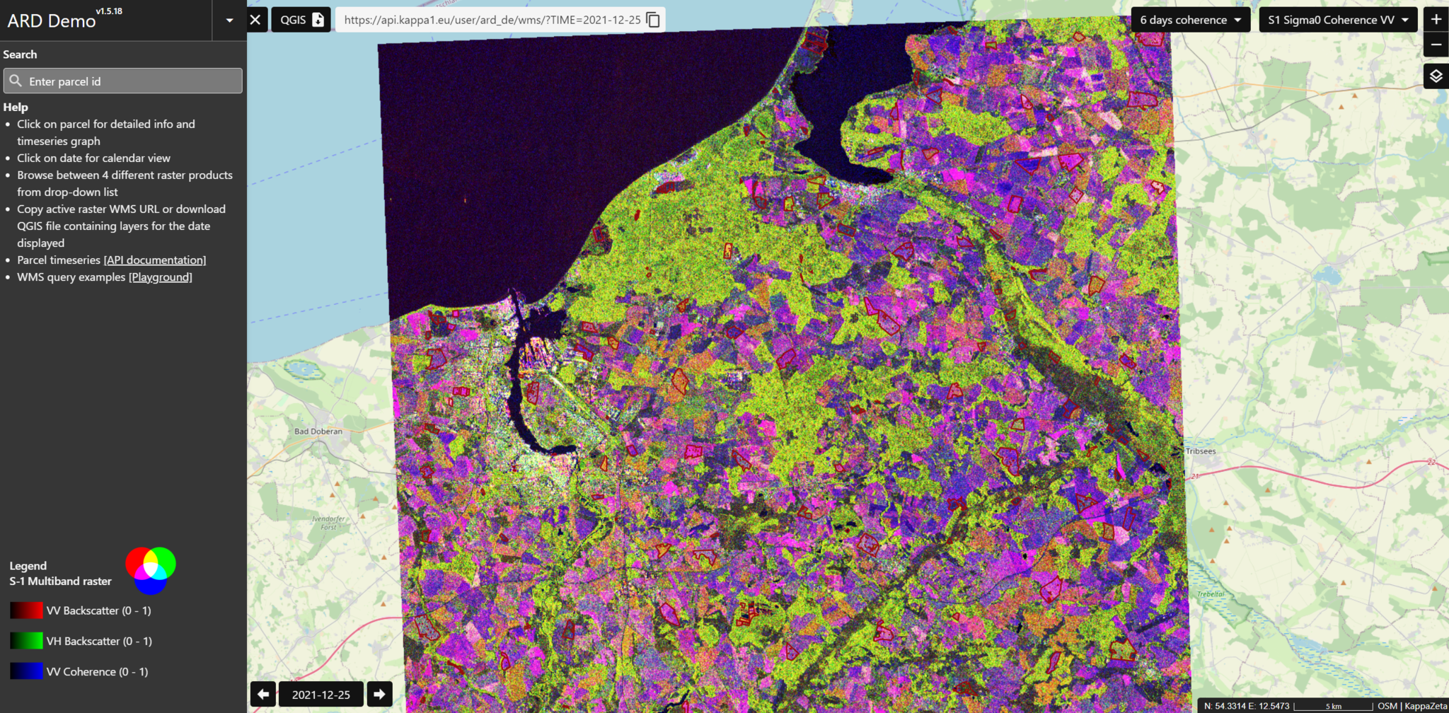
Why do we need Sentinel-1 data service?

Satellite data is still not widely used, because it can be complex to acquire and work with. However, the Copernicus Earth Observation programme is a great way to look at our planet and its environment, as it provides continuous radar and optical imagery with its Sentinel satellite missions (currently 1, 2, 3, 5p and 6).

Still, especially Sentinel-1 radar data is used by relatively small user segments, including university research groups and some specific GIS/EO applications. For example, Estonian Environment Agency has recently started to use Sentinel-1 data for complementing ice map for both Baltic Sea and larger Estonian lakes, https://jaakaart.envir.ee/.

The Sentinel-1 data is different than most other satellite data because it is not dependent on weather or daylight, and thus is able to provide data on days where other satellites cannot because of clouds. 

As Sentinel-1 is a great data source acquiring large quantitites of Synthetic Aperture Radar data with global coverage, which is valuable for numerous Earth Observation applications, we have decided to make it accessible and easy to use for a wider audience.  

Figure 1. Example of standard Sentinel-1 GRD backscatter image


There are some services on the market, which make optical satellite data, like Sentinel-2 or Landsat easy to use and analyse. However, there is no application that utilizes the Sentinel-1 data in its full potential. Therefore, KappaZeta team decided to resolve this issue by establishing the KappaOne service, where S1 data will be processed and prepared for the user in analysis ready data (ARD) format.  

What is KappaOne?

KappaOne stands for one-click or one API command integration. There are six Sentinel-1 ARD products available, which are presented in human-friendly as well as machine-readable form, providing value for a long list of end-user applications. 

Provided Sentinel-1 ARD layers are the following:

  • Time series of small geographical region – parcel, statistics (mean, median, min, max, stddev) of Vertical-Horizontal (VH) and Vertical-Vertical (VV) backscatter, VH/VV backscatter ratio, VH and VV 6-day repeat pass coherence (phase difference changes);

  • Calibrated high-resolution VH and VV repeat pass interferometric coherence rasters;

  • Calibrated high-resolution VH and VV backscatter and VH/VV ratio rasters;

  • Multi-polarisation backscatter image for visual use as a WMS service;

  • Synthetic Sentinel-2-like natural colours image based on Sentinel-1 and -2 time series with AI-modelling;

  • Synthetic NDVI-like raster based on Sentinel-1 and -2 time series with AI-modelling. 

You can have an overview of our service here. This is a web-map, where you can choose the layer which you are interested in. Moreover, you can scroll the dates in the calendar to see how the area of interest looked in a particular time.  

Figure 2. KappaOne web-map

The other convenient feature of our webpage is the one-click command with which you can download a pre-set QGIS project for the layer and date you are interested in. You can open the setup file in QGIS, where you will see the WMS layer with the chosen product for a particular date. 

Another asset of the KappaOne service, is a visualisation of the time series of parcel-level statistics. By clicking on the parcel of interest, the chart of the area becomes visible, where you can browse the time series of various Sentinel-1 and Sentinel-2 parameters.

Who can use it and where?

There are numerous applications where Sentinel-1 Analysis Ready Data could be used. For example, this service can be used by the EO or GIS companies without Synthetic Aperture Radar expertise for Mapping/GIS analysis tasks, where frequent and systematic data is needed. 

Sentinel-1 ARD is vital also for the agricultural subsidy checks, where on-spot checks conducted by the inspectors are gradually replaced by satellite monitoring. The grassland maintenance checks can be very slow and expensive if done manually. Therefore, for this kind of task, the usage of satellite monitoring is a great way of saving time and money. 

With Sentinel-1 data many more tasks can be solved. As it was underlined before, satellite monitoring is an efficient tool for resolving various measurement and assessment tasks, where instead of gut feeling decisions could be done based on actual data. It can be used for the greenhouse gas fluxes modelling, as well as flood risk assessments or the landscape dynamics based on historical data and damage mapping near real time. Also, the monitoring of the seaports could be performed, which would reflect the flow of the sea containers. 

The Figure below shows Sentinel-1 multiband image for the port area in Rostock, Germany. Yellow areas on the image represent big metallic constructions, which are the sea containers transported with ships. It is visible that on 29th of May 2021, the ship was leaving or entering the port and ships had changed their location in Rostock port and its surrounding in the sea by 4th of June.

Figure 3. Example of changes in the port, visible on S1 multiband image, a) 29.05.2021, b) 04.06.2021


Figure 4 illustrates the ploughing example on the Synthetic NDVI layer, which is computed from Sentinel-1 raster with usage of historical Sentinel-2 data. It is visible that the vegetation index before ploughing on the parcels is significantly higher than after ploughing, as the color changes rapidly from yellow to dark orange.  

Figure 4. Example of ploughing event, visible on S1 sNDVI, a) 29.05.2021, b) 04.06.2021

Olga Wold

Geospatial data quality specialist

olga.wold@kappazeta.ee

Read more

Free and open AI-based cloud mask for Sentinel-2

Asking a person on the street ‘what is a cloud mask and why would one need it’, you would probably receive more questions than answers.  Yet people who have worked with EO data for at least a year, or, even better, who have tried to program an automatic classifier, know exactly what we are talking about.

Sentinel-2 is a beautiful European data factory, producing tons of valuable imagery every day. Its full potential is yet to be exploited. The first Sentinel-2 satellite was launched in 2015 and after launching the second satellite (2B) the system reached its full data production capacity in the second half of 2017. One of the factors limiting the usage of Sentinel-2 data is clouds. There is a need for an accurate mask for separating the clear pixels from the corrupted ones. Figure 1 illustrates it well – not only the cloud covered areas are unusable for great majority of EO applications, but also the cloud shadows cause trouble. If you run e.g. a crop classification algorithm on these regions you cannot expect an adequate result.

Figure 1. Cumulus clouds and cloud shadows on Sentinel-2 satellite image

While Sentinel-2 system, functioning as a data factory, is beautiful and undeniably a huge game changer, then the official Sen2cor cloud mask incorporated to the L2A data products can be insufficient in terms of accuracy when used in fully automatic processing chains. The issues rise with underestimating the cloud shadows and small fragmented clouds. While feeding an operational processing chain (such as the grassland mowing detection system of KZ) with this data a lot of corrupted pixels are passed through, deteriorating the accuracy of the end result. In practice we have ended up with aggressive outer buffering and few other post-processing steps to reduce the errors. But obviously these are all just work-arounds without solving the underlying problem. The cloud mask itself, out-of-the-box, should be accurate enough without thinking about it during the work processes.

When digging deeper, you find that the Sen2cor cloud mask processor has a rule-based thresholding decision tree with some post-processing steps (e.g. morphological filtering to reduce the noise). On one hand it is impressive how accurate results this decision tree is able to produce in a global scale, but after the revolution of AI and deep learning one knows that the same task can be solved much better with a different – more modern design.

Leaving the Sen2cor cloud mask as it is, the proposal of KappaZeta was convincing enough that we were given a chance to develop an AI-based Sentinel-2 cloud mask for ESA and we are very grateful for it.

Which other cloud masks are out there?

Firstly, we would like to outline how import is to develop open source cloud masks. There are a few privately developed cloud masks, raising the first question about accuracy figures. If these details are not public, it is also hard to assess how good the offered product really is and that raises many other questions. Furthermore, this adds to the unnecessary amount of time spent on something that could be shared openly, reducing duplication, and contributing to improved products. Therefore, everybody would win time-wise and quality-wise from more open approach and sharing. This is what we believe in and hope that more and more companies over time will come to the same conclusion.

One of the best open source cloud masks is probably s2cloudless by Sinergise. Find more information from here, here and here.

There is just one thing we would like to question and open for discussion. They write that: “We believe that machine learning algorithms which can take into account the context such as semantic segmentation using convolutional neural networks (see this preprint for overview) will ultimately achieve the best results among single-scene cloud detection algorithms. However, due to the high computational complexity of such models and related costs they are not yet used in large scale production.” So CNNs are great, but too heavy to be practical? Let us put this claim in doubt, at least in 2020. One thing is CNN model fitting, which for a complex model can be computationally expensive, that is true. But the other thing is running a prediction with a pre-trained model. This is much cheaper – and this is what you need to do when you put a CNN into production.

One of the best research papers on using deep learning for cloud masking is probably by DLR. We are taking this as one of the starting points for our development. They claim higher accuracies than Fmask (which is roughly on the same level with Sen2Cor) at a reasonable computational cost (2.8 s/Mpix on a NVIDIA M4000 GPU).

There are also several CNN-based cloud masking research papers by the University of Valencia. E.g. by Mateo-García and Gómez-Chova (2018) and Mateo-García, Gómez-Chova and Camps-Valls (2017).

All in all – deep learning as a universal mimicking machine has proven to be at least as accurate in recognizing objects from images and segmenting them semantically as human interpreters. Deep learning has been proven in various domains with image interpretation, speech recognition and, text translation. Computer Vision, which focuses particularly on digital images and videos, has enormous success in medical field, where data labelling is an expensive procedure or rapidly developing autonomous driving cars field, where huge amount of data should be processed in real time. There is every reason to believe that it will excel also in detecting clouds and cloud-shadows from satellite imagery. What determines the success is the quality and variety of the model fitting reference data set.

We believe that cloud masking is such an universal pre-processing step for satellite imagery that sooner or later someone will develop an open source deep learning cloud mask and all the closed source cloud masks become obsolete. Let us then try to be among the first and help the community further.

How?

The goal of the project is to develop the most accurate cloud mask for Sentinel-2. We know it is going to be hard and to avoid going crazy by trying to solve everything at once, we are limiting the scope of the project. We concentrate on Northern European terrestrial summer season conditions. With Northern Europe we mean the area north from the Alps, which has relatively similar nature and land cover. Summer season means the vegetative season – from April to October. We start from terrestrial conditions (with all due respect to the marine researchers), because we believe it has higher impact for developing operational services that make clients happy, for example in the agricultural and forestry sectors.

Everyone, who has worked on machine learning projects, know that the most critical factor for success is the quality and variety of input data. In our case it is the labelled Sentinel-2 imagery following the classification schema agreed in CMIX. Eventually each pixel should have a label, one out of four: 1) clear, 2) cloud, 3) semi-transparent cloud, 4) cloud shadow. For labelling we are using CVAT with a few scripts for automation and thanks to the hard work of our intern Fariha we have already labelled more than 1500 Sentinel-2 cropped 512x512 pixels tiles. The work goes on to have a large and accurate reference set for CNN model fitting.

To be more effective, there are several machine learning techniques we are going to apply:

1) Active learning. To select only the tiles and pixels, which have the highest impact for increasing the accuracy of the model. Labelling is a time-consuming process, and it is critical to do only work that matters.

2) Transfer learning. The idea is to use all possible open sources labelled Sentinel-2 images to train the network and then fine-tune it on our smaller focused dataset.

The initial literature review is completed and we plan to start with applying U-Net on our existing labelled dataset. We still have many open questions, e.g. should we use one of the rule-based masks as an input feature; is the improvement worth the fear that the network can possibly capture the same errors; to what extent we can augment existing features in terms of brightness and angles; can certain calculated S2 coefficients help the network, such as NDVI, NDWI etc?

Last, but not least, it is an open source project. All our results, final software and source code will be freely and openly distributed in GitHub. Openness and accessibility of our software should directly translate into greater usage. We are also intending to learn from the community and take advantage of the existing open source projects and labelled cloud mask reference data sets.

If you have any good suggestions how we could improve our cloud mask or be aware of some parallel developments for cooperation, please let us know. Our project runs from October 2020 to September 2021.

Further information:
Marharyta Domnich
marharyta.dekret@kappazeta.ee

Read more

Data splitting challenge

Almost any machine learning pipeline requires an input data split for training and validation purposes. However, ground truth collection is challenging and could be gathered from different sources. Various sources provide different confidence levels for the labels and in general it would be beneficial to test the model on the most confident samples, but also providing some part of it for training as well, keeping the class distributions as uniform as possible. We are facing the challenge of having unbiased data split with adjustable filters in different tasks and it feels that there is a need for a more general solution or brainstorming from the community.

Mowing detection

One of the examples where we meet the splitting challenge is the mowing detection task. The goal of mowing detection is to predict the time at which the grass on the field was cut. Thus, as part of our mowing detection project, each year we collect field books from farmers and field reports from the inspectors of the local paying agency. The received data is converted and reviewed manually, and some of the ground truth is produced from the manual labelling.

The labels would differ in trustworthiness, depending on the source (farmer field books, inspector field reports, any of the former with manually adjusted dates, or fully manual labelling). Since inspector field reports are the most reliable source, we would use most of them for the validation and test set. However, we would need at least some of them to be present in the training dataset as well. Additionally, each dataset is expected to have as well balanced classes distribution as possible, perhaps with additional filtering to randomly drop least trustworthy samples from the over-represented class.

Considering the aforementioned conditions, let’s say we would like to have 70% of the labelled data for training, 20% for validation and 10% for testing. For validation and testing, we would only use instances from inspector field reports and farmer field books with tweaked dates. For training, we would use data from all sources, including the ones from inspector field reports and tweaked field books which were left over from the test and validation datasets.

Crop classification

Another task we are dealing with is crop classification. We would like to detect the crop type of agricultural fields out of 28 possible classes. Similarly to the mowing detection we have different sources for labels, some of which have been provided by the local Agricultural Registers and Information Board, some from drone observations. For crop classification, class balance distribution plays the core role. In order to mitigate the issue of an unbalanced dataset, undersampling and oversampling can be used. Undersampling and oversampling should be available for the training subset, while for testing we would use some of the fields with labels of high confidence. Some of the classes might have a poor representation, due to which general split ratios might leave the validation or test dataset without any samples, whereas we need to ensure that all datasets have enough samples.

Image credit: Madis Ajaots

Thus, the requirements for splitting are the following. We would like to have 70% / 20% / 10% splits, ensuring that for smaller representing classes at least one instance is present in all sets. Additionally for the test set we would like to have the list of high confidence instances together with random leftover samples that added up to 10% of the whole data.

Generic and configurable

While such processing chains can be implemented, we have found it tricky to have it generic and configurable enough to cater for all sorts of projects with different (and sometimes rapidly changing) requirements.

Current solution

Currently we have separate implementations for mowing detection and crop classification, both of which take input parameters from a config file. The config file is basically python code and supports the definition of custom filter functions for datasets. For each dataset, the current solution invokes custom filters (if any) and then performs random sampling of data indices, leaving the rest of the samples for the next datasets. The samples which have been filtered out, are also left for the next datasets, for each dataset might have a different filter.

The reason why we prefer to use data / sample indices instead of data directly, is to have a layer of abstraction. This way the splitting logic could be agnostic of data type. It would not matter whether a single sample / instance is a raster image, an image time-series or time-series of parameter values which have been averaged over a pre-defined geometry.

For multiclass applications such as crop classification, data indices are sampled separately for each class within each dataset. The splitting also supports capping of samples for classes which are represented too well. However, if there are too few samples per class, a low threshold can be applied such that a different split ratio would be used. For instance, in the case of 70% training, 20% validation and 10% testing dataset with just 9 samples in one of the classes, we might end up with 7 samples in the training dataset, 2 samples in validation and 0 in the test set. To mitigate the issue, we could have the ratios adjusted to 40% training, 30% validation and 30% testing for classes with less than 100 samples.


Ideas for future developments

Instead of project-specific implementation of the splitting logic, we would prefer to have a generic framework for graph-based data splitting with support for cross-validation and bagging. Please let us know if there is such a framework already out there, or if there would be community interest in developing the framework.

Read more

Towards the operational service of crop classification

We are about to finish a R&D project, where we developed and tested crop classification methodology specifically suited for Estonian agricultural, ecological and climatic conditions. We relied mostly on Sentinel-1 and -2 data and used neural network machine learning approach to distinguish 28 different crop types. Results are promising and the methodology is ready for operational service to automate another part of agricultural monitoring.

Using machine learning in crop type classification is not new, and definitely not a revolutionary breakthrough - already for decades different classifiers (Support Vector Machine, Decision Trees, Random Forest and many more) have been used in land cover classification. Recently also neural networks, the wunderkind of machine learning and image recognition, are widely used in crop discrimination. Satellite data, as the main input to classification models, has no serious alternatives, since our aim is to implement it on worldwide scale and in applications, which run near real time. So, why even get excited about another crop type classification study, which exploits same methods and datasets as tens of previous studies?

I can give you one reason. Estonia has been very successful in following European Commission (EC) guidelines and rules in modernizing the EU Common Agricultural Policy. In 2018 EC adopted new rules that allow to completely replace physical checks on farms with a system of automated checks based on analysis of Earth observation data. The same year Estonian Agricultural Registers And Information Board (ARIB) launched the first nation-wide fully automated mowing detection system, which uses Sentinel-1 and Sentinel-2 data and where the prediction model inside the system is developed by KappaZeta. The system has been running for 3 years, it has significantly reduced the amount of on-site checks and increased the detection of non-compliances. In short – saved Estonian and EU taxpayers’ money. Automated crop discrimination is the next step in pursuing the above-mentioned vision and will probably become the foundation of all agricultural monitoring. With proved and tested methodology, it’s highly likely that Estonia will take this next step in the very near future and launch it again on the nationwide level. This is definitely a perspective to be excited about.

Now, let’s see how we tackled “the good old” crop classification task.

Input data

Although algorithms and methods are important to make a difference in prediction model performance, the training data is the most valuable player in this game. In Estonia all farmers who want to be eligible for subsidies need to declare crops online (field geometry + crop type label). This open dataset is freely accessible to everyone and has the permission to re-use and redistribute both commercial and non-commercial purposes. Since the crop type labels are defined by farmers and most of them are not double-checked by ARIB, there can be mistakes (according to ARIB’s estimations, less than 5%). Therefore, for additional validation we ran our own cluster analysis on time-series to filter out obvious outliers in each class.

After we had the parcels and labels, we calculated time-series of different satellite-based, plus some ground-based features (precipitation, average temperatures, soil type). When extracting features from satellite images there are two ways to go: pixel- or parcel-based extraction. We selected the latter and averaged pixel values over the parcel to obtain one numerical feature value per statistic for each point in time (see Figure 1).
Figure 1. An example time-series of one Sentinel-1 feature (cohvh - 6-day coherence in the VH polarization) for one parcel.

For Sentinel-1 images preprocessing we have developed our own processing chain to produce reliable time-series for several features. From the previous studies it’s known that features (channel values and indexes) from Sentinel-2 images combined with features from Sentinel-1 images (coherence, backscatter) give better classification results than any of these features separately.

Figure 2. The whole dataset can be imagined as a three-dimensional tensor with the feature parameters on one axis, parameter statistics on another, and date-time on the third axis.

We used data from 2018 and 2019 seasons (altogether more than 200 000 parcels) and aggregated all crop type labels into 28 classes which were defined by the need of the ARIB.

Model architecture

Figure 3. Model architecture.
Due to the very unbalanced dataset we had to under-sample some classes and over-sample others for the training data. In small classes we used the existing time-series and added noise for data augmentation.

Model architecture was rather simple – input layer, flatten layer, three fully connected dense layers (two of them followed by batch normalization layer) and output (Figure 3). Our experiment with adding 1D CNN layer after input didn’t improve results significantly. More complicated ResNet (residual neural network) architecture increased training time by approx. 30%, but results were similar to a linear neural network.


Classification results

F1 score on validation set (9% of all dataset) was 0.85 and on test set (2% of all dataset) 0.84. In 10 classes the recall was more than 0.9 and in 16 classes more than 0.8. See more from Figure 4 and 5. 
Figure 4. Test set results.
Figure 5. Normalized confusion matrix of the crop classification results (recall values).

Some features are more important than others

In a near-real time operative system our model and feature extraction would have to be as efficient as possible. For an R&D project we could easily calculate 20+ features from satellite images, feed them all to the model and let the machines compute. But what if not all features are equally important?

They are not. We found that the 5 most important features are Sentinel-1 backscatter (s1_s0vh, s1_s0vv), NDVI, TC Vegetation and PSRI from Sentinel-2. To our surprise, soil type and precipitation sum before satellite image acquisition had low relevance.

The 5 most important features played different role during the season – Sentinel-2 features were more important in the beginning and in the end of the season, while Sentinel-1 features had more effect during mid-season.
Figure 6. Importance of different features in crop classification, estimated using Random Forest.

What next?

This project was part of a much larger initiative called “National Program for Addressing Socio-Economic Challenges through R&D. Using remote sensing data in favor of the public sector services.” Several research groups all over Estonia worked on prototypes to use remote sensing in fields like detecting forest fire hazard, mapping floods and monitoring urban construction. Now its up to Estonia’s public sector institutions to take the initiative and turn prototypes into operational services. With this work we have proved, that satellite-based crop classification in Estonia is possible, accurate enough and ready to be implemented as the next monitoring service for ARIB.

If you are more interested about this study, our Sentinel-1 processing pipeline or machine learning expertise, then feel free to get in touch. We have the mentality to share not hide our experience and learn together on this exciting journey.

Read more

Open access to ALOS-2 radar satellite data?

End of previous year (2019) Japan announced that the Japan Aerospace Exploration Agency (JAXA) will be providing open access to information and data from a suite of their radar satellites (original statement here). To be more specific, free and open access to the wide-swath observation data from the L-band radar satellites, ALOS (ALOS/AVINIR-2, PALSAR) and ALOS-2 (ALOS-2/ScanSAR) will be made available. The price of ScanSAR images is at the moment around 700 euros.

ALOS-2 spacecraft in orbit (image credit: JAXA)

The Japanese space and satellite program consist of two series of satellites – those used mainly for Earth observation and others for communication and positioning. There are 3 Earth Observation satellites in nominal phase, 3 in latter phase in operation and 3 more under development.

Greenhouse gases Observing SATellite-2 "IBUKI-2" (GOSAT-2) is measuring global CO2 and CH4 distribution of lower and upper atmosphere. Climate "SHIKISAI" (GCOM-C) satellite carries an optical sensor capable of multi-channel observation at wavelengths from near-UV to thermal infrared wavelengths (380nm to 12µm) to execute global, long-term observation of the Earth’s environment. Advanced Land Observing Satellite-2 "DAICHI-2" (ALOS-2) aims are to monitor disaster areas, cultivated areas and contribute to cartography.  

ALOS-2, which is specifically interesting for radar enthusiasts, is a follow-on mission from the ALOS “DAICHI”. Launched in 2006, ALOS was one of the largest Earth observation satellites ever developed and had 3 different sensors aboard: PRISM (Panchromatic Remote-sensing Instrument for Stereo Mapping) for digital elevation mapping, AVNIR-2 (Advanced Visible and Near Infrared Radiometer type 2) for precise land coverage observation and PALSAR (Phased Array type L-band Synthetic Aperture Radar) for day-and-night and all-weather land observation. ALOS operations were completed in 2011, after it had been operated for over 5 years.  

ALOS-2 was launched in 2014 and carries only radar instrument aboard. New optical satellite, ALOS-3, which will improve ground resolution by approx. three times from that of ALOS (2.5 to 0.8 m at nadir, wide-swath of 70 km at nadir), is already under development together with ALOS-4, which will take over from ALOS-2 to improve the functionality and performance.  

Let’s come back to present day. The state-of-the-art L-band Synthetic Aperture Radar (PALSAR-2) aboard ALOS-2 have enhanced performance compared to its predecessor. It has a right-and-left looking function and can acquire data in three different observation modes:

  • Spotlight – spatial resolution 1x3 m, NESZ -24, swath 25 km. 
  • Stripmap – spatial resolution 3-10 m, swath 30–70 km. Consist of Ultrafine (3 m), High sensitive (6 m) and Fine (10 m) modes. 
  • ScanSAR – spatial resolution 60-100 m, swath 350–490 km.  

PALSAR-2  specifications (images credit: JAXA)

Emergency observations have highest priority for ALOS-2, but for systematic observations Basic Observation Scenario (BOS) has been developed. This ensures spatial and temporal consistency at global scales and adequate revisit frequency.  ALOS-2 BOS has separate plans for Japan and for the rest of the world, success rate for these acquisitions is 70–80 %.  

PALSAR-2  observation modes (images credit: JAXA)

Basic observations over Japan are mostly undertaken in Stripmap Ultrafine mode and sea ice observations during winter in ScanSAR mode.

Stripmap Fine and ScanSAR modes are used for global BOS. There are several areas of interest, where ALOS-2 is putting more focus, for example:

  • Wetlands and rapid deforestation regions in ScanSAR mode
  • Crustal deformation regions both in Stripmap Fine and ScanSAR mode
  • Polar regions both in Stripmap Fine and ScanSAR mode

In addition to those special regions global land areas are observed in Stripmap Fine mode at least once per year.

We made a little experiment to test, how many acquisitions we get over city of Tartu per year. Here are the results (platform for viewing and ordering data is here):


Screenshot from Earth Observation Data Utilization Promotion Platform.
YearNumber of images per year
2015
6
20167
20179
20188
20197

So, compared to Sentinel-1 radar-satellite, ALOS-2 acquisitions frequency is much lower over Europe, and its difficult to develop agriculture monitoring services only on this platform. For forestry and other environmental monitoring, where changes are not happing that often as in agriculture, ALOS-2 can be very useful due to its better spatial resolution than Sentinel-1. Being an L-band satellite it can also penetrate deeper into vegetation and provide information about the lower layers of the canopy. JAXA is already developing ALOS-4 with PALSAR-3 aboard, which will aim broader observation swath compared to the predecessor.

Read more

Overview of new RADARSAT Constellation Mission

Exciting remote sensing news from last year. Canadian Space Agency has launched new generation of Earth observation satellites called The RADARSAT Constellation Mission (RCM) on June 12, 2019 aboard a SpaceX Falcon 9 rocket. It became operational in December 2019 and provides data continuity to RADARSAT-1 (not operational anymore) and RADARSAT-2 (still operational) users.
Illustration of the three RCM satellites on the same orbital plane. Image credit: Canadian Space Agency

RCM is a combination of three identical and equally spaced satellites, flying in the same orbit plane 32 minutes apart at an altitude of 600 km. Each of the spacecraft carries Synthetic Aperture Radar (SAR) aboard, plus a secondary sensor for Automatic Identification System (AIS) for ships. When RADARSAT-2 has left- and right-looking operation, then RCM is only right-looking, because multiple satellites increase revisit times and eliminate the need to look both ways. The SAR device aboard RCM satellites is quite similar to RADARSAT-2 – C-Band antenna, 100 MHz bandwidth, 4 regular polarization modes (HH, VV, HV, VH) plus compact polarimetry.  Polarization isolation is slightly better: >30 dB. See detailed comparison of RADARSAT satellites here.

The constellation system provides better coverage with smaller and less expensive satellites. This configuration allows for daily revisits of Canada’s territory, as well as daily access to 90% of the world’s surface. RCM can provide a four-day exact revisit (3 satellites equally phased in a 12 day repeat cycle orbit), allowing coherent change detection with InSAR. For specific applications (ship detection, maritime surveillance) data latency from acquisition to delivery can be only 10-30 minutes, but in general it will be from hours to 1 day.

RCM has several observation modes, but the mission is primarily designed for medium-resolution monitoring:

  • Low resolution (100 m), swath 500 km, NESZ -22 dB
  • Medium resolution (16, 30, 50 m), swath 30-350 km, NESZ -25…-22 dB
  • High and very high resolution (3-5 m), swath 20-30 km, NESZ -17..-19 dB
  • Spotlight (1x3 m), swath 20 km, NESZ -17 dB
    RADARSAT Constellation Mission observation modes. Image credit: Canadian Space Agency.


Read more

Base Camp Hackathon 2020

KZ extended team during hackaton
In the beginning of March our team participated Base Camp Spring 2020 hackaton organized by Garage48 and Superangel.
Our aim was to develop prototype for our time series API sandbox and map customer segments. Long weekend was successful and besides great mentoring, new ideas and contacts, we won the runner-up prize "Superangel’s Support on Steroids package".
Base Camp Hackathon is an exclusive hackathon format, designed for young startups that already have a working prototype. Latest edition took place from 6th to 8th of March 2020 in Tallinn, Estonia and 12 teams, Kappazeta among them, were invited to develop their prototypes or products even further. For this 3-day event Teet Laja and Raja Azmir joined our team to help us out in front-end development and business analysis.

The results? During the productive weekend we conducted couple of possible users interviews to validate the new product idea and created landing page to test our concept and capture contacts of interested people. 
Also a simple API Sandbox was created, where potential customers have the chance to test core possibilities of our service. We are not yet there to provide world-wide near real time Sentinel-1 time series API, but we are moving towards there and improving our process chain rapidly. Next step is to take whole process to cloud platform (DIAS), to be closer to input satellite data and boost performance. Exciting times! 
Read more